Alhadi B
Department of Mathematics, Faculty of Mathematics and Natural
Science
University of Indonesia, Depok (16424) - INDONESIA. Phone/Fax:
62-21-7863439.
Ponidi
Department of Mathematics, Faculty of Mathematics and Natural Science
University of Indonesia, Depok (16424) - INDONESIA. Phone/Fax: 62-21-7863439.
Recently, the computer-aided software has been used intensively in many courses in mathematics, especially in computational subject such as to solve initial value and boundary value problems in PDE. We have used many software packages in student's lab assignment, such as FORTRAN, PASCAL, MATLAB, MATHEMATICA, and MAPLE in order to accelerate their understanding in concept and to improve their computational skill. Regarding our last few year evaluations in our PDE course, we conclude that Maple is the most effective one in solving, comparing and visualization of numerical and exact solution in PDE. PDE is one of obliged course for Pure Mathematics and Computational Mathematics student.
In this paper, we will focus our discussion on computational project to solve, to compare and to visualize the solution of the heat, wave and Laplace's equation in PDE in our course class. We have arranged our course materials in effective ways by combining lecturing in class before midterm with lab assignment, discussion and final project after midterm. To make more effective and efficient class, we grouped the class and arranged the member of group by mixed-up them base on their major skill, theoretical (Pure Mathematics student) and computational (Computational Mathematics student).
As the result we found the increasing of academic atmosphere among the student. It can be detected with more enthusiastic and involving students in their group or individual assignments. Beside that, we see that MAPLE is comfortable and interesting to be used in our mathematics course, especially in PDE. The student also have new experienced and perception about modeling, solving methods, visualization, and real interpretation on PDE Problems.
1. INTRODUCTION
Department of Mathematics, University of Indonesia has five majors of study program such as Pure Mathematics, Statistical Mathematics, Computational Mathematics, Operation Research and Actuarial Mathematics. The curriculum for each study program consists of obliged and elected course. Partial Differential Equation (PDE) is an elected course in this department for the student who has taken the Ordinary Differential Equation (ODE) course, but it is an obliged course for Pure Mathematics and Computational Mathematics students.
PDE is an interesting and relevant course regarding the wide area of its application in modeling of many natural phenomena. Various methods to obtain the solutions are discussed in this course, which are separated into two ways, exact solution techniques and numerical approximation techniques. Both solutions can be simulated and visualized by using suitable computer-aided software. The obtained solutions, including its simulation and visualization can be used to interpret the model of its natural phenomena, according to the objectives of the problems.
Previously, various teaching methods have been implemented by some lecturers of the department in this course mainly by using traditional teaching method that explaining the theory in the class without any computer-aided treatments. Since 1995's the teaching method in this course has been improved by giving lab assignment with MATLAB but it was still in limited number of computers. In 1998 the department has been granted QUE project from World Bank, a prestigious project in Indonesia for improving the quality of undergraduate education programs. The project is available for five years (1998-2002) and covering many components that can be used or improved such as staff development, laboratory equipment, teaching equipment, library equipment, building renovation, furniture, consumable, technical assistance and staff incentive. Therefore the department has been procuring large quantity of new hardware, software and textbook & journal, so with these new procurements many courses in the department have been improved in their teaching methods and enriched with new material and new lab assignment packages, including in the PDE course. In addition, after considering the capability of MAPLE in solving and visualizing the exact solutions and numerical approximations of PDE, this software was used as the new practical software tool for student's lab assignment in PDE course in this department.
The objective or this paper is to give an alternative method in improving of PDE course learning, base on our first experience in implementing this new learning method in PDE course that had been implemented in even session of 1998/1999 semester's period in Department of Mathematics, University of Indonesia. In this paper, the discussion are focused on student's lab assignment on computational project in solving, comparing and visualizing the solution of PDE for some natural phenomena such as the heat, wave and Lapace's equation. The course materials have been arranged in effective ways by combining lecturing process in class before midterm; and giving student's lab assignment, discussion and final project after midterm. To make more effective and efficient class, we grouped the class and arranged the member of group by mixed-up them base on their major skill, theoretical (Pure Mathematics student) and computational (Computational Mathematics student).
Considering all above descriptions, the paper will be arranged in the following order. After introduction as section 1, with covering the backgrounds, the objectives, the methods and the structure of the paper; in section 2 will be given the lesson plan which consists of the objectives of learning process, learning contents, learning method and any supporting media. The core issue of the paper is about lab assignment that will be explained in section 3. Finally, the conclusion will be stated at final section.
2. LESSON PLAN
The general instructional objective of the course is to encourage the student ability and skill in understanding concept and method for solving some major issues in PDE model and its application in physics. Details of learning material and its objective are showed at table 1.
|
No |
Learning Materials |
Learning Objectives |
Weeks |
|
1 |
Introduction: It covered the definition of PDE, order and solution, and PDEs construction by elimination the arbitrary constants or functions of a surface family. |
The students will understand the definition of PDE, order and the kind of its solutions. Furthermore, base on the family of surfaces which are contain of arbitrary of parameters or functions, they will be able to construct the PDEs by elimination of its parameter or function |
1 |
|
2 |
PDE of order one: It consists of linear and nonlinear Partial Differential Equations of order one. |
The students will understand the definition of PDE of order one, how to find the general and complete solution of linear PDE of order one, and by Charpit method they can solve the nonlinear PDE of order one |
2,3 |
|
3 |
PDE of higher order: It consists of homogenous and non-homogenous PDE of higher order with constant coefficients. |
The students will understand the definition of homogenous and non-homogenous PDE of higher order with constant coefficients, and can obtain its solutions |
4,5 |
|
4 |
PDE of order two with variable coefficients: It consists of special types and Laplace's transform of PDE of order two with variable coefficients and nonlinear PDE of order two. |
The students can find the solutions of special types of PDE of order two with variable coefficients, convert complex PDE of order two with variable coefficients to another simpler form by using Laplace's transform. Furthermore, they can solve the nonlinear PDE of order two |
6,7 |
|
5 |
Mid test |
To evaluate student's mastering of learning materials and objectives |
8 |
|
6 |
Applications of parabolic, hyperbolic, and elliptic PDE of order two with variable coefficients: It covered various exact and numerical methods to solve the PDE of order two with variable coefficients. |
The students will understand the definition of parabolic, hyperbolic and elliptic PDE of order two with variable coefficients. By separate of variable, D'Alembert and Fourier Analysis methods, they can find the exact solutions of this PDE. Furthermore, they can find the numerical approximation solution by finite difference methods. Finally by using computer-aided software, they can simulate, visualize and compare the both solutions |
9-15 (*) |
|
7 |
Final Test |
To evaluate student's mastering all of learning materials and objectives of this course |
16 |
Table 1: Learning Materials and Its Objectives
(*) The student's activities will mainly be focused in lab with their lab assignments.
The process of teaching and learning of this course have been arranged in two sections. The first section is done from the beginning of semester until midterm test. This section is focused in developing the general concept and analytical skill in solving various issues in PDE. The second section is done after midterm of semester until final test. This section is focused in building practical skill in solving, simulating, visualizing, interpreting and reporting the solutions of PDE in some physical problems. The process of teaching and learning used the combination of lecturing in class in first section and student's lab assignment, discussion, report presentation and doing final project in second section. To make more effective and efficient class, we grouped the class and arranged the member of group by mixed-up them base on their major skill, theoretical (Pure Mathematics student) and computational (Computational Mathematics student).
The evaluation process is done for both students and lecturer. The students is evaluated by using some evaluation items that have been involved along teaching and learning process in both section 1 and section 2 period of course. These evaluation items are midterm and final test results; lab assignment grades; student's group grades; and student's homework and activities. The lecturer is evaluated by giving questioner to the students about technique of presentation; class interaction; consultation and counseling time outside the class; discipline of lecturing time and its lesson plan; quality and availability of textbook references; relevancy of course material with the others courses; assignments, homework and examinations.
3. STUDENT'S LAB ASSIGNMENTS
Laboratory of Computational Mathematics, University of Indonesia has been improved its facilities regarding QUE project granted since 1998. In 1998, the lab has received 38 sets of new PC-HP8 Vectra with Pentium-II processor and multimedia through this project. All of them are running in WindowsNT 4.0 operating system and connected to WindowsNT server using HP8200. Beside that, the new released software for mathematical & statistical programming tools like MATLAB, MAPLE, SPSS and another language programming like C-language, VisualBasic are also procured in 1998. Nowadays, we have just proposed to buy 20 sets of new PC-Compaq Deskpro with Pentium-III processor and multimedia, including new released software in mathematical & operation research programming like Scientific Workplace, LINGO. The department proposes to continue in improving lab facilities until the end of the project.
Previously, some lecturer had used MATLAB for student's lab assignment programming tools in PDE course in this department. Base on this experience, we found the weaknesses of this software such as It can not determine the exact solutions of PDE in symbolic forms, it is difficult enough to generate and to show PDE function in comfortable forms, it has a limited library for solving and simulating PDE model. So MAPLE have been chosen to replace MATLAB for student's lab assignment tools in PDE course in this department, because of it can covers the previous weaknesses. Beside that MAPLE is more comfortable and easy to be used in determining, simulating and visualizing both the exact and numerical solutions. Finally, by using new powerful hardware and software from QUE project the activities in student's lab assignment run more valuable and useable than before.
There are six sessions proposed in student's lab assignment schedule and it is arranged to practice the application topics of PDE in physics. Before practicing session in the lab, the students are also discussed the topics and presented it at the class discussion session. Beside the arranged schedule, the students who still have not familiar enough with MAPLE can attend the assistance sessions supporting by lab assistance staff. The assignment materials and objectives can be seen at table 2.
|
No |
Assignment Materials |
Assignments Objectives |
Weeks |
|
1 |
Introduction to MAPLE: It covered the introducing of basic programming skill and libraries of MAPLE, the basic techniques for finding exact and numerical solutions of PDE. |
The students can make program with MAPLE to generate PDE models and implement the chosen algorithms to solve the model to find the exact and numerical solutions. They utilize MAPLE library in discovering the exact solutions and setup finite difference methods in finding numerical approximation solutions. At the end, they can visualize the graph of both solutions. |
9 |
|
2 |
One-dimensional Heat Equations with Initial and Boundary Values. |
The students can understand the process and background concept to construct and solve one-dimensional heat equations model with initial and boundary conditions. (**) |
10 |
|
3 |
Two-dimensional Heat Equations for Steady-state Conditions with Initial and Boundary Values. |
The students can understand the process and background concept to construct and solve two-dimensional heat equations for steady-state conditions with initial and boundary values. (**) |
11 |
|
4 |
Two-dimensional Heat Equation for Unsteady-state Conditions with Initial and Boundary Values. |
The students can understand the process and background concept to construct and solve two-dimensional heat equations for unsteady-state conditions with initial and boundary values. (**) |
12 |
|
5 |
Wave Equation with Boundary Values. |
The students can understand the process and background concept to construct and solve wave equation with boundary values. The students use D'Alembert and Fourier Analysis methods to transform and simplify the model in applying finite difference algorithms. (**) |
13 |
|
6 |
Final Project |
To evaluate and to extend the achievement of student's activities, all of the students must build their own PDE model as improvisation of all previous given models. At the end, the student must make the report to summarize all of previous given PDE models and its solving methods. |
14 |
Table 2: Student's Lab Assignment Materials and Objectives
(**) Mainly objectives of these lab assignments, the students can solve the given model with MAPLE to find the exact solutions and to practice various finite difference methods to find the numerical approximation solutions. At the end, the students can visualize the graph of both solutions, compare and analyze them in various initial and boundary conditions.
All of the lab sessions are done by groups, except for final project. The members of each group are combined the students from Pure Mathematics, who have good in theoretical concepts with the students from Computational Mathematics, who have good in programming. Its combinations will make the group more powerful and effective. The example of the results of student's lab assignment can be observed at the appendix of this paper. At the end of all lab sessions, the students report that it is more easy and comfortable to find the solutions of PDE models by using numerical approximation methods. The exact solutions are difficult enough to be determined, actually by using manual analytical methods. Furthermore, by simulating and visualizing the model in various initial and boundary values the students will have new point of views about PDE models and its solutions. They will get more realistic interpretation and perception about the solutions, related to its natural phenomena in physics.
4. CONCLUSIONS
Every good learning process must covers three essential aspects of learning process such as orientation, implementation and evaluation. All of the components have been tried be achieved better in this course, not only in every class meeting but also in the whole parts of the course. As the result, the positive responses were received from student's feedback after using and implementing the above learning method in PDE course in Department of Mathematics, University of Indonesia. Moreover, the academic atmosphere among the student and lecturers are increasing. It can be detected with more enthusiastic and involving students in their group or individual assignments. Beside that, we see that MAPLE, which has capability to solve both symbolic and numeric solutions, is more powerful, comfortable and interesting to be used in our mathematics course, especially in PDE. The student also have new experienced and perception about modeling, solving methods, visualization, and real interpretation on PDE Problems. Actually this method must be improved toward as well as the improvement of new technology and supporting media in learning process in order to make the students more enthusiastic and enjoyable and to establish better academic atmosphere.
REFERENCES
Wylie & Barret, Advance Mathematical Engeneering, Mc Graw Hill,1995.
Erwin Kreyszig, Advance Mathematical Engeneering, John Willey & Sons,1997.
A. Jeffrey, Linear Algebra and Ordinary Differential Equations, Blackwell Sc. Publ., 1990.
Paul Du Chateau & David Zackman, Applied Partial Differential Equations, Harper&Rev, 1989.
Donald W Trims, Applied Partial Differential Equations, PWS Publ. Co, Boston, 1990.
David Blecker & George CS, Basic Partial Differential Equations, PWS Publ. Co, Boston, 1990.
Walter Garder JH, Solving Problems in Scientific Computing Using Maple and Matlab, 3rd ed, Springer Verlag, 1997.
Software and Manual: Maple.
APPENDIX
A Simple Example of Student's Lab Assignment Problems and Result
PROBLEM (in Session 5):
Wave Equations with Initial and Boundary Values
Let the heat equations form is:
Utt(x,t) - Uxx(x,t) 0, 0<x<1, 0<t ...(1)
with boundary and initial values:
U(0,t) U(1,t) = 0, 0<t
U(x,0) sin Õ x, 0 = < x < 1
A. The exact Solution:
Let U(x,t) =F(x+t) + G(x-t)
So U(x,0) F(x) + G(x) = sin
Õ x ...(a)Ut(x,t) F'(x+t) - G'(x-t)
Ut(x,0) F'(x) - G'(x) = 0 = ...(b)
The derivative of equation (a) is:
F'(x) + G'(x) cos
Õ x. = ...(c)Form equation (b) it shows that:
F'(x) G'(x)
After substitution to equation (c), it forms:
F'(x) G'(x) = 1/2 cos
xSo F(x) 1/2 sin
Õ x +C1, and G(x) 1/2 sin Õ x + C2It proved that the exact solution of equation (1) is:
U(x,t) 1/2 sin
Õ = (x+t) + 1/2 sin Õ = (x-t) sin (Õ x) = cos (Õ t) ...(2)B. The Numerical Solutions:
Let the equation (1) is modified to:
Utt(x,t) - 4 Uxx(x,t) 0, = 0<x<1, 0<t
with initial and boundary values:
U(x,0) sin
Õ x, 0 = < x <1Ut(x,0) 0, 0 < x = < 1
U(0,t) U(1,t) = 0, 0 < t
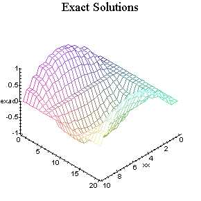
So, base on equation (2), the exact solution is: =
U(x,t) sin (
Õ x) = cos (2Õ t)By using D'Alembert Method (with m 10, N = 20, T 1 and
a = 2),So the numerical solutions in MAPLE 5.0 = are:
|
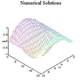
> = restart: >=m: 10:T:=1:N:=20:l:=1:alpha:=2: /*numerical solutions*/ > w:=array(0..m,0..N): >=h: l/m:k:=T/N:lambda:=(k*alpha)/h: > g:=x->0:f:=x->sin(Pi*x): > for j from 1 to N do w[0,j]:=0: w[m,j]:=0: od: w[0,0]:=f(0):w[m,0]:=f(l): > for i from 1 to m-1 do w[i,0]:=f(i*h): w[i,1]:=(1-lambda^2)*f(i*h)+(lambda^2)/2*(f((i+1)*h)+= f((i-1)*h))+k*g(i*h): od: > for j from 1 to N-1 do for i from 1 to m-1 do w[i,j+1]:=2*(1-lambda^2)*w[i,j]+lambda^2*(w[i+1,j]+w[= i-1,j])-w[i,j-1]: od; od: Numerical Solutions |
/*exact solutions*/ > eksak:=array(0..m,0..N): > for j from 0 to N do > t := j*k: > for i from 0 to m do x:= i*h: eksak[i,j]:=sin(Pi*x)*cos(2*Pi*t); od; od: > with(plots): > for j from 0 to N do for n from 0 to m do pa:=(n,j)->w[n,j]; pb:=(n,j)->eksak[n,j] od; od; > setoptions3d(title=`Numerical Solutions`); > = plot3d(pa,0..m,0..N,axes framed,labels=[xx,tt,ww]); > setoptions3d(title=`Exact Solutions`); > = plot3d(pb,0..m,0..N,axes framed,labels=[xx,tt,exact]); Exact Solutions |
The comparison of the solution results on several points:
First iteration
|
x |
t |
Numeric (i,1) |
Exact(i,1) |
|
0.00 |
0.05 |
0 |
0 |
|
0.10 |
0.05 |
.2938926260 |
.2938926263 |
|
0.20 |
0.05 |
.5590169945 |
.5590169944 |
|
0.30 |
0.05 |
.7694208840 |
.7694208845 |
|
0.40 |
0.05 |
.9045084973 |
.9045084973 |
|
0.50 |
0.05 |
.9510565160 |
.9510565160 |
|
0.60 |
0.05 |
.9045084973 |
.9045084973 |
|
0.70 |
0.05 |
.7694208840 |
.7694208845 |
|
0.80 |
0.05 |
.5590169945 |
.5590169944 |
|
0.90 |
0.05 |
.2938926260 |
.2938926263 |
|
1.00 |
0.05 |
0 |
0 |
Last iteration
|
x |
t |
Numeric (i,20) |
Exact(i,20) |
|
0.00 |
1 |
0 |
0 |
|
0.10 |
1 |
.3090169945 |
.3090169945 |
|
0.20 |
1 |
.5877852520 |
.5877852520 |
|
0.30 |
1 |
.8090169945 |
.8090169945 |
|
0.40 |
1 |
.9510565160 |
.9510565160 |
|
0.50 |
1 |
1. |
1. |
|
0.60 |
1 |
.9510565160 |
.9510565160 |
|
0.70 |
1 |
.8090169945 |
.800169945 |
|
0.80 |
1 |
.5877852520 |
.5877852520 |
|
0.90 |
1 |
.3090169945 |
.3090169945 |
|
1.00 |
1 |
0 |
0 |
The visualization of the solutions:
Picture A.1: Graphics of both numeric and exact solutions: